σ, SF, ASF, RSF, and e-RSF
| σ, SF, ASF, and RSF
Menu-Links |
Photoionization Cross-sections, σ, and
|
|
|
The photoionization cross-section, σ, is the primary fundamental parameter determining XPS peak intensities. It represents the probability of a photon, of given energy, causing an electron to be completely removed (i.e. ionization) from a given atomic orbital of a given atom.
Absolute σ values have been calculated from theory for a wide range of X-Ray energies for all atomic orbitals (energy levels) of every element in the periodic table. For practical use in XPS, σ is usually normalized relative to the values of either C1s or F1s defined as unity (1). At 1486.6 ev (Al Kα source) σ for F1s is theoretically 4.43 greater than that of C1s, meaning that for identical concentrations of C and F atoms, a given photon flux would remove 4.43 times as many F1s electrons as C1s electrons. The second fundamental factor concerns the KE distribution of the photoelectrons produced by ionization from a specific atomic orbital. If photoemission was exclusively a one electron process, meaning all other electrons in the system remained unchanged by the production of the core-level hole, then all the intensity would go into a single peak at the KE corresponding to the orbital energy of the electron concerned. In reality, other (valence region) electrons interact with the hole generated, and this will steal intensity from the “main” peak (defined here as the lowest BE component), putting it into “satellite“ peaks (multiplet splittings and shake-up peaks) that appear at lower KE than the main peak. Because valence region electrons are involved, the degree to which this occurs will likely be chemistry dependent. One may be able to ignore satellite intensities when the level of accuracy concerned is low, but for elements with open shell d or f valence electrons in their compounds (actually a large part of the periodic table) the losses from the main peak can be substantial and therefore the fraction remaining, termed y, much less than 1, particularly for solids.
Calculated σ values refer to the total intensity integrated
|
|
| Contributed by C. R. Brundle (USA) – Continued below |
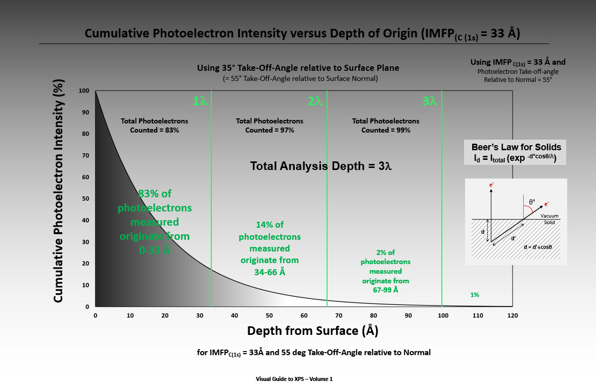
After initial generation, photoelectrons in a solid have to pass through the solid to escape and be detected. They may be inelastically scattered on the way, losing energy and so be removed from the intrinsic photoemission peak and appear somewhere in the background to lower KE after that peak. The fraction lost this way is dependent on the value for the Mean Free Path Length, λ, for inelastic scattering, which is dependent on the KE of the photoelectron, and the material being traveled through.
The KE dependence has been experimentally determined, and also calculated, and is well understood (2). λ is proportional to KE~0.66, so the low KE end of a given spectrum has a shorter λ and therefore loses more intensity from the photoemission peak and samples less depth than the high end.
Sensitivity Factors, SFs, in XPS are empirically derived factors (from compounds of known composition) by which peak intensity is normalized (divided by) to provide an atomic concentration, atom% (3). The intensity observed for the “main” peak, I, is dependent on the fundamental parameters above, but also on several experimental parameters specific to the instrument being used.
I = nSF = nσyλ[FTφ]
n is the atomic concentration of the element concerned. F is the X-Ray flux, T is the instrument Transmission Factor, φ is an angular distribution factor, which depends on the angle between the X-Ray source and the detector, the nature of the orbital concerned ( s, p, d or f ), and the atomic number of the atom.
In modern instruments, T is either “corrected at source”, so that it has a value of unity (1) throughout the generated spectrum, or can be so corrected by the software afterwards. F drops out if comparing intensities in a given spectrum (which is nearly always the case in XPS).
φ is unity for all s orbitals, and also for all orbitals of all elements when measured at the Magic Angle of 54.6 deg. Though the variation of φ for gas phase atoms and molecules has been well understood for decades (4), there is not much evidence of significant variation in solids (where theory is confused by elastic scattering, which changes the direction of of an emitted electron), so is either set at 1, or is known to be 1 if the measurement is at the magic angle.
Therefore, a Relative Sensitivity Factor, RSF, for ionization from any orbital of any atom, is relative to C1s, defined as unity, is given by:
RSF = σyλ/yC1sλC1s = σyKE0.66/yC1s KEC1s0.66 = σy[KE/KEC1s] 0.66/yC1s
If one assumes y is the same for all elements, then this reduces to:
RSF = σ[KE/KEC1s]0.66
Using this above equation, an empirically derived σ for any orbital can be easily extracted from the RSF and compared to the theoretical value.
The spreadsheet shown below gives an in depth comparison between theory and empirical measurements for σ made by different authors (Crist and Mack), both using a Thermo K-Alpha instrument, under the above assumptions and at or near the magic angle. Both authors tried to include only intensity from a main peak, except when not possible because of peak overlap, or glaringly obvious large satellites nearby.
The Crist table of “IP-e-SFs” (periodic table format) presents two of what Crist considers the most reliable sets of values measured from freshly exposed bulk of single crystals of binary compounds for many of the elements.
In contrast, the Mack SF numbers were extracted from a 2017 Thermo database filled with adjusted Scofield values, which have no explanation or report of what compounds were used or how they were prepared to adjust which Scofield values.
Large discrepancies between Scofield, Crist and Mack SFs may be due to one or more of the following:
- The chemical compounds being used not having the expected composition in the near surface depth actually being probed by XPS.
- y actually varying substantially (yC1s may be varying too) from compound to compound and for differing atomic orbitals for a given atom (theoretically expected )
- Inadequacy of background subtraction
- Real errors in the theoretical calculations
References
- J. H. Scofield, J. Elec. Spec. 8 129 (1976)
- S. Tanuma, C. Powell, and D. R. Penn, Surf. Interface Anal. 47, 871, (2015)
- C. D.Wagner, et al, Surf. Interface Anal. 3, 211 (1981)
- F. Reilman, A. Msezane and S. R. Manson, J. Elec. Spec. 8, 389, (1975)
- P. Mack, Thermo Scientific, 2017 version of MS-Access database interfaced to Avantage software stored in Bin directory of Thermo K-alpha XPS instrument
- B. V. Crist, XPS International, (private communication, 6 month project using cleaved, freshly exposed bulk of man-made binary single crystals, freshly exposed bulk of natural crystals, very high purity grains, beads, or powders)
Crist IP e-SF Periodic Table – Aug 30 2019 (PDF)
(Click on Title or Image to open Current Version of IP-e-SF Table)
After opening the PDF, ZOOM in (expand) the PDF by 300-400% to see e-SF values clearly!


Scofield Calculated Photoionization Cross-Sections (σ)
Sensitivity Factors (SFs), Normalized to C (1s)=1.0
In this table, the photoionization cross-sections (σ) calculated by Scofield have been normalized to give an SF for C (1s) = 1.0. His calculations are based on a central field potential model.

Validation Test of Scofield SFs

Comparison of Scofield SFs, Thermo’s Modified Scofield SFs, & Crist’s Modified Scofield SFs (Graphic Plots)


Table Based Version:
Comparison of Scofield SFs, Thermo’s Modified Scofield SFs, &
Crist’s Modified Scofield SFs


Periodic Table of Calculated IMFPs (TPP2) for
Principal XPS Signals

Trendline for Photoelectron IMFP vs KE of Emitted Photoelectrons
Used to modify Sensitivity Factors or Atomic Sensitivity Factors to Correct for IMFP Effects. Exponent is 0.6659, (0.67).

Photoelectron Intensity versus Depth of Origin
Using C (1s) IMFP = 33 Angstroms and a 35 deg electron take-off-angle with respect to plane of surface.
Comparison of PHI ASFs to Scofield SFs
We have forgotten to remove the IMFP in these two plots.


Kratos SFs for Mg X-rays (<1990)

Biesinger’s SFs for Monochromatic Aluminum X-rays
Kratos Axis Ultra and Kratos Axis Nova XPS Instruments


Perkin-Elmer (now Ulvac-PHI) RSFs (not ASFs)
for a Omni-Focus Electron Lens with a 54.7 deg Magic Angle and a monochromatic Aluminum X-ray source

Wagner’s ASFs with F (1s) = 1.0 (published 1980)
Using a Varian IEE and Perkin-Elmer 550 XPS Instruments (not using HSA)
