Bad Peak-fits Published in Journals – Explained
Bad Peak-fits Accepted by Reviewers for Publication
found by Image Search for XPS spectra
First, please think about these Questions!
Why do we collect high energy resolution, chemical state spectra?
Why do we peak-fit those chemical state spectra? Goal?
How will we use the chemical state assignments from peak-fitting?
How important are the relative percentages of the peaks in the peak-fit?
What happens if we make wrong chemical state assignments?
Do we need to constrain peak areas? FWHMs? BEs? G:L ratios?
Bad Peak-fits Published in Literaturefrom Image search for XPS spectra. |
||
ExplanationWhy is this a Bad Peak-fit? |
Bad Peak-fits Accepted by Reviewers! |
How to improve this peak-fit |
|
|
|
|
| Cr (2p3) Peak-fit – Published in Journal | Cr (2p3) Peak-fit – Published in Journal | Cr (2p3) Peak-fit – Published in Journal |
| Three (3) of the four (4) peaks appear at reasonable BE positions, but there are no BEs or FWHMs. The Cr 4+ peak is reported in SSS to appear at 576.4 eV which is 1 eV higher than the assigned peak.
The Cr (0) peak can have a asymmetric tail on the high BE side due to valence-core interactions, but it should not have Lorentzian tail on low BE side. Peaks have different amounts of Lorentzian shapes. Chemical compounds seldom have a large Lorentzian shape % such as that seen for the Cr(OH)2- peak. The peak-shapes for the 3 compounds should be the same unless there is something unusual present. The Cr (0) peak max should not be above the data points of the actual spectrum. The spectrum fit envelop is drawn with a very thin line and is difficult to see. Peak ID “Cr(2p) is missing. |
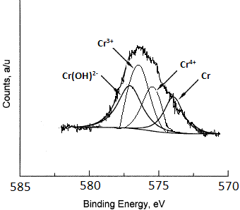 |
2-3X more scans gives better S/N and information.
Use same Gaussian-Lorentzian peak-shapes for the 3 compounds. Add BEs, FWHMs, and relative %s Make the envelop line thicker. Include a Chi-square value on the spectrum and also include a residual plot at the bottom of the plot. To help check the accuracy of the BE values, it would be useful to include small tick marks representing 0.5 eV steps. A calibration BE and the date instrument calibration was last checked would be useful to read. The XPS signal name “Cr (2p)” should be added to the top right corner of the plot. The name of the chemical being analyzed should be added. |
|
|
|
|
| Al (2p) Peak-fit – Published in Journal | Al (2p) Peak-fit – Published in Journal | Al (2p) Peak-fit – Published in Journal |
| S/N is extremely poor. Can barely see peaks. The chemical state assignments used here appear at, or close to, the BEs to which they are assigned if hydrocarbon C (1s) appears at 284.8 eV, but it is impossible to resolve 8 different chemical states from a spectrum region that has only 22-24 data-points. If true, each peak has only 3 data-points.
This spectrum has no background, no synthetic peaks, and no peak envelop. This is enough reason to ignore or reject this spectrum and the chemical states that are assigned to noise spikes. A normal single peak will have between 15-20 data-points, not 1-3 shown here. The spectrum has too much noise to be useful. If typical smoothing is applied, the spectrum will become “wavy” and is still meaningless. XPS signals from a laboratory XPS never produce FWHM that are <0.2 eV. Chemical compounds of Aluminum normally have FWHM >1.5 eV. A pure metal Al (2p) peak has a FWHM >0.8 eV, not 0.2 eV as indicated here. This spectrum has at 3 real XPS peaks which have peak maxima at ~74 eV, 76 eV, and 78 eV with FWHM that are ~1.5 eV wide. The scientist who made these chemical state assignments ignored the peak at ~76 eV, and 78 eV which must have chemical state assignments because they account for >60% of the total signal. It is possible that the sample has all 8 of these chemical states, but without peak-fitting, it is impossible to decide what is present or what is absent. |
 |
50-100X more scans or use a larger Pass Energy. If PE was very small such as PE=10 or 20, then that is a waster of time because the energy resolution does not need to be that high for insulators usually.
The data-analyst who made these assignments was probably just having fun, and testing to see if the reviewer or the professor would notice the many bad aspects of this plot. If this was a real plot of an XPS spectrum of Al (2p), then it must have less noise, a background, synthetic peaks, FWHM values >1.3 eV, BE values, and a peak envelop. If this is a real spectrum, then the scientist must explain or give a label that identifies the peaks that occur at 76 and 78 eV. The XPS signal name “Al (2p)” should be added to the top right corner of the plot. The name of the chemical being analyzed should be added. |
|
|
|
|
| O (1s) Peak-fit – Published in Journal | O (1s) Peak-fit – Published in Journal | O (1s) Peak-fit – Published in Journal |
| Peak ID “O (1s)” is missing. S/N should be better.
FWHM are different. One is 2.0 eV and the other is 2.5 eV. This is acceptable if the difference is based on pure chemical state data, but both are larger than the typical maximum O (1s) FWHM, 1.8 eV. The plot does not include chemical state assignments. A third peak should have been added at ~535 eV and identified, so the raw data do not match the peak envelop. This region is not due to differential charging because it appears on the high BE side of the peak, not the low BE side. |
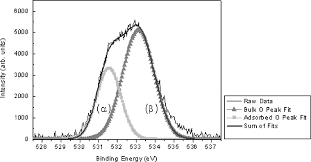 |
2-3x more scans would improve S/N
Check that charge control gives narrow peak for PE polymer. Maybe use a 2X smaller PE. Chemical state assignments would help the reader. BEs, FWHMs, and relative %s should be added. The FWHM are large, indicating that the sample is not properly charge controlled. An explanation about the missing peak should be added. The XPS signal name “Cr (2p)” should be added to the top right corner of the plot. BE axis is normally plotted right to left. The name of the chemical being analyzed should be added. |
|
|
|
|
| S (2p) Peak-fit – Published in Journal | S (2p) Peak-fit – Published in Journal | S (2p) Peak-fit – Published in Journal |
| Peak ID “S (2p)” is missing. S/N is not so good.
The Li2S peak should have 2p3 and 2p1 peaks separated by 1.2 eV with a 2:1 peak area ratio. The S-C peak has the same problem. The same problem exists for the peak at ~163 eV. All peaks use significant level of Lorentzian peak shape which is not used for insulators. Lorentzian is useful for conductors and gases. The peak area envelop that contains peak areas from the synthetic peaks poorly matches the real spectrum. The Chi-square for this spectrum should be >10 or >20. The background goes beyond the actual spectrum. The endpoint for the upper end should have been ~174 eV. This caused a high chi-square value. |
 |
To resolve this many peaks, the S/N needs to be 5x higher.
The XPS signal name “S (2p)” should be added to the top right corner of the plot. BE axis is normally plotted right to left. For insulators, the G:L ratio is usually 80:20 but can sometimes be 90:10, or 70:30. BEs, FWHMs, Relative %s, and Peak area ratios should appear on this plot. |
|
|
|
|
| N (1s) Peak-fit – Published in Journal | N (1s) Peak-fit – Published in Journal | N (1s) Peak-fit – Published in Journal |
| The bright green wavy line has no meaning but is labelled with “Fresh” and “organic matrix”.
The FWHM are all < 1 eV which is not typical for Nitride peaks or organic nitrogen peaks. The FWHM is different for all 4 peaks by 20+%. N-Sn and N-Ti assignments are pointing at the same peak. The text should have an explanation about this overlap. There are two overlapping peak envelops which has no meaning. The green one is probably the envelop. The purple line is probably the raw data after too much smoothing. The arrow from the 1000 hrs label can not be understood. The BE axis is not traditional, right to left, so it is confusing to study. |
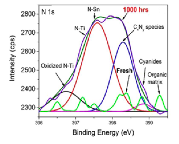 |
Smoothing should be much much less, if any. It is always better to have good S/N from more scans even though it takes more time.
The FWHM are small because the data was smoothed too much. Better to use a larger pass energy if you need to avoid noise. Peak labels for chemical states is useful to have on a plot. The plot is missing BEs, FWHMs, and relative %s. |
|
|
|
|
| Ca (2p) and Ni (2p) Peak-fit – Published in Journal | Ca (2p) and Ni (2p) Peak-fit – Published in Journal | Ca (2p) and Ni (2p) Peak-fit – Published in Journal |
| Ca (2p) Plot
Based on the BEs in the literature in the NIST SRD20 database of BEs, Ca(OH)2 has the same BE as CaO. The CaCO3 BE is ~0.5 eV greater than the be of CaO or Ca(OH)2. The literature BEs do not agree with these assignments. Pyrolysis normally causes water (H2O) to be lost from hydroxides, producing either an oxide or a carbonate if CO2 is present in the pyrolysis chamber, The errors are most likely due to charging effects and charge referencing issues. The different spin-orbit peaks are not labelled. Inexperienced scientists will not understand the extra peaks that are not labelled. BEs, FWHMs, and relative peak areas are missing. The spin-orbit “Ca(2p)” label is missing.
Ni (2p) Plot The noisy red line at the base has no meaning and should not be there. The dark blue line is the Background. The FWHM of Ni and NiO are <0.8 eV which are meaningless. NiOOH is claimed to be present, but it is most likely a Multiplet Splitting peak due to the Ni(OH)2. There is no signal label. There are no BEs, FWHMs, or relative peak %s. |
 |
The energy resolution and S/N ratios of these spectra are good and allows reader to understand the data and the assignments.
The Ni (2p) plot should be expand to show only the Ni (2p3) signal so we can see the NiO and Ni peaks more easily. Both spectra need signal labels, BEs, FWHMs, and relative peak areas. Both spectra, Ca (2p) and Ni (2p) suffer from wrong peak assignments. To prove that such species exist at the BE defined requires the analyst to collect data from pure samples of those materials and not to depend on the BEs listed in the NIST database. BEs are plotted in the traditional way, from right to left. |
|
|
|
|
| C (1s) Peak-fit – Published in Journal | C (1s) Peak-fit – Published in Journal | C (1s) Peak-fit – Published in Journal |
| The raw spectra data are not shown. The peak envelop is very smooth, indicating excessive smoothing. The BEs for the C-C and C-O peaks are close to expected. The C=O and O=C-O peaks are too high by ~ 1 eV. The C=O and O=C-O FWHM are 2X larger than the C-C and C-O peaks. Unless there is some known data, all FWHM should be the same +/-15% or less. This wrong BEs and 2X larger BEs for the C=O and O=C-O peaks are hiding other chemical states, that include a carbonate and maybe a bi-carbonate. The Background line is missing. No BEs or FWHMs are shown. |  |
Do not hide raw spectra data because it looks like the scientist synthesized the spectra by using a plotting software or Excel. The C (1s) plot also hides the raw spectra. The peak positions and chemical state assignments are reasonable.
It would be useful to expand the spectra by 5-10 eV more. All FWHM in the right side C (1s) spectrum are reasonable. |
|
|
|
|
| S (2p) Peak-fit – Published in Journal | S (2p) Peak-fit – Published in Journal | S (2p) Peak-fit – Published in Journal |
| The peak at ~168.5 eV is not a Satellite. It is the sulfate (SO4) species that is present in this sample. This peak also has a 2p3 and 2p1 component.
The two peaks, S 2p3 and S 2p1, are due to the sulfide (S 2-) species in this sample. The 2p3 to 2p1 peak area ratio is 2:1, but there are no relative peak %s so we can not know if that is used. The background is a linear background which shows there is a lot of signal not accounted for between the sulfide and sulfate peaks of the raw data. All 3 peaks use an excessive amount of Lorentzian peak-shape, which was probably intended to produce a better fit.
|
 |
An iterated Shirley background would produce a better fit.
BEs and FWHM should be added. The name of the chemical being analyzed should be added. |
|
|
|
|
| Ca (2p) Peak-fit – Published in Journal | Ca (2p) Peak-fit – Published in Journal | Ca (2p) Peak-fit – Published in Journal |
| The BE values are not linear. The 354 eV label should be 352 eV, and the 358 eV label should be 356 eV. The energy difference between Ca 2p3 and 2p3 is 3.6 eV.
This spectrum has two XPS peaks. One peak at ~348 eV is due to the Ca (2p3) spin-orbit electrons and the second peak at ~353 eV is due to the Ca (2p1) spin-orbit electrons. The are spin-orbit coupled. Both signals should have the same number of synthetic peaks for correct peak-fitting. The background should not end up in between two spin-orbit related peaks. The background should end at ~357 eV, not at 351 eV. These 3 minerals, Aragonite, Calcite and Vaterite, are different crystalline forms of CaCO3. XPS is seldom able to discern differences in crystalline forms. There is no indication that this spectrum is from a powder or a mixed crystal. If all three species are present, then they would have nearly identical Ca (2p3) BEs. Zeolites are aluminosilicates (AlSiOx) that can be modified to include Ca, Na, K etc. Ca(NO3)2 has a Ca (2p3) BE that might occur near 348.4 eV but a Ca zeolite does not.
|
  |
The data is nice looking data. The data-analyst needs to correct the BE scale and make a proper background.
The data-analyst should use XRD to determine the ratio of the 3 different crystalline forms if they are present. |
|
|
|
|
| Cr (2p) Peak-fit – Published in Journal | Cr (2p) Peak-fit – Published in Journal | Cr (2p) Peak-fit – Published in Journal |
| This plot does not identify the element or spin-orbit. This plot does not list BEs, chemical states, FWHMs, or constraints. Based on the BEs, this is a Cr (2p) spectrum.
At the low BE side of peak-fitted peak there is a very wide synthetic peak at ~575 eV. On the other peak that is not peak-fitted there is a very similar feature at ~585 eV. These two very wide synthetic peaks are due to differential charging, and should not be assigned to the presence of elemental Cr. This peak-fit style has been used to peak-fit XPS signals that have multiplet splittings. Multiplet splittings do not necessarily have the same FWHM for each of the synthetic peaks. The same is true for BE shifts. |
 |
This plot should be labelled as Cr (2p3) because the Cr (2p1) is not peak-fit. The data-analyst should have noticed the wide peaks at low BE on not only these two peaks, but also the O (1s).
Many papers publish only one of several chemical state spectra, and do not include the survey spectrum. To prove the purity of the sample, the author should include the survey spectrum and other key spectra such as O (1s) or C (1s). C (1s) of contamination helps to establish BE calibration even though the C (1s) BE does not appear at 284.8 or 285.0 eV. |
|
|
|
|
| N (1s) Peak-fit – Published in Journal | N (1s) Peak-fit – Published in Journal | N (1s) Peak-fit – Published in Journal |
| This is a N (1s) spectrum which is not labelled. We know by looking at the BE axis. The FWHM, BEs and relative %s are not labelled. Chemical states are not labelled.
The spectrum range at the top is truncated to 10 eV, but the other two spectra have 14 eV wide spectra. In general, the minimum width for any spectrum is 20 eV. It seems the author is hiding some peak in the top spectrum by limiting the spectrum to 10 eV range. This implies deception and bad science. The synthetic peak at ~400 eV is too wide. It should be fit with 2 peaks. The FWHM for 3 of the peaks is ~1.5 eV which is reasonable for organic types of Nitrogen. If a peak appeared at 397 eV or lower it would be assigned as a Nitride and the FWHM would be ~1.0 eV. The very wide, FWHM ~4 eV, peak at ~404 eV should be fit with 3-4 more synthetic peaks which are due to various NOx species.
|
 |
These spectra should have been run using a 20 eV window range at a minimum. A 25-30 eV width would allow the reader to learn more from the actual spectra.
Again, add BEs, FWHM, and relative peaks%s. S/N looks good until you look at the N (IV) peak at 404 eV. A 3-4x higher S/N might reveal the presence of peaks and shoulders in this very wide peak. Energy resolution is good. If you use a much smaller Pass Energy, then you must collect 10x more scans. |
|
|
|
|
| Ru (3d) Peak-fit – Published in Journal | Ru (3d) Peak-fit – Published in Journal | Ru (3d) Peak-fit – Published in Journal |
| This is a good set of spectra. Survey and Ru (3d). There are still two issues with the Ru (3d) plot. Carbon C (1s) overlaps the Ru (3d3) so there should be a synthetic peak for C (1s) at ~285 eV. The (3d) spin-orbit pair has a 6:4 ratio, but the peaks (blue and purple lines) dedicated to metallic Ru do not match that ratio. Tje peak at ~285.8 eV is due to an overlap of Carbon contamination and the RuO2 peak (3d3). The peak area of the green line (RuO2, 3d5) must show a RuO2, 3d3, peak with the 6:4 ratio.
This means that there are two missing peaks. |
 |
The labelling is good, but BEs and FWHM are missing. Relative area % is missing.
To change this into a great peak-fit, the data-analyst needs to add the 2-3 peaks that must replace the gold colored peak. |
|
|
|
|
| B (1s) Peak-fit – Published in Journal | B (1s) Peak-fit – Published in Journal | B (1s) Peak-fit – Published in Journal |
| Based on the BEs, his plot displays 2 B (1s) and 2 N (1s) peak-fits. If the peak labels were larger, the reader would understand the data without eye strain.
The BN spectra at the top are good, but the B (1s) and N (1s) spectra at the bottom have low BE tails that is typical for differential charging. The FWHM of these two peaks is also 30+% wider than the two at the top, which is most likely due to differential charging. The FWHM in the bottom spectra are radically different with no reason. If the survey spectrum was provided, it would be easy to better understand this data. |
 |
BEs, and FWHMs should be added. The C (1s) and O (1s) spectra should be added because they would reveal if the sample is or is not suffering differential charging. All high res chemical state spectra will have similar low BE tails if differential charging is present. |
|
|
|
|
| O (1s) Peak-fit – Published in Journal | O (1s) Peak-fit – Published in Journal | O (1s) Peak-fit – Published in Journal |
| The FWHM for O (1s) for many materials is between 1.5-1.8 eV. Various carbonates have FWHM >2. All of these O (1s) peaks are >2.0 eV. One is >3 eV.
The most obvious problem here is that the data-analyst has used a straight line for all backgrounds, and has made no attempt to overlap the raw data and the straight line. This might be due to the use of a very simple plotting software, such as Excel. When a peak FWHM is larger than usual, the data-analyst must add another peak even though it may be difficult to assign a chemical state to that new peak. If the data-analyst realizes that the data is suffering from differential charging which might make peaks broader than normal, then a new set of spectra are needed if you want to have correct information. The BEs, FWHMs and relative areas are not documented on the plot. A chemical name should be included. The X-axis should be reversed. |
 |
To improve these plots, the background needs to be adjusted so it overlaps the actual data points.
A 3rd peak needs to be added at ~531.5 eV to all 4 spectra. The proposed chemical state of each peak should be added to the plots. S/N is good. If the scientist really wants more information from the O (1s) peaks, then the Pass Energy should be decreased by 2x, and the number of scans need to be increased by 5-10x. In this manner the spectrum may reveal clear shoulders. |
|
|
|
|
| S (2p) Peak-fit – Published in Journal | S (2p) Peak-fit – Published in Journal | S (2p) Peak-fit – Published in Journal |
| The S (2p) signal has a spin-orbit pair of peaks that are 1.2 eV apart and have a 2:1 peak area ratio. This spectrum shows a 2p (1/2) peak that is roughly 7X larger than the 2p (3/2) peak which is not possible.
The peak at ~163 eV is very broad (~2.5 eV). This BE range is due to Sulfides and it is possible that the sample has 2 types of sulfides. The peak at ~164 eV could be due to a S-S single bond. The peak at 169 eV is a Sulfate type of sulfur. It is not a Satellite peak unless there is some metal signal nearby. The use of Lorentzian peak shape hides the shoulder that confirms the presence another peak. The background is a Shirley type of background but it is reversed so it is not a useful background. |
 |
|
|
|
|
|
| N (1s), O (1s) Peak-fits – Published in Journal | N (1s), O (1s) Peak-fits – Published in Journal | N (1s), O (1s) Peak-fits – Published in Journal |
 |
||
|
|
|
|
| C (1s), O (1s) Peak-fits – Published in Journal | C (1s), O (1s) Peak-fits – Published in Journal | C (1s), O (1s) Peak-fits – Published in Journal |
 |
||
|
|
|
|
| Cd (3d), S (2p) Peak-fits – Published in Journal | Cd (3d), S (2p) Peak-fits – Published in Journal | Cd (3d), S (2p) Peak-fits – Published in Journal |
 |
||
|
|
|
|
| Zr (3d), P (2p) Peak-fits – Published in Journal | ||
 |
||
|
|
|
|